About Me

• Graduated from Monash University with Bachelors of Commerce in 2018
• Currently a Masters Student at the University of Melbourne

Why R Markdown

Hypothesis testing

Bayesian Estimation and Graphical presentation

Demonstration of Reproducible report

Case Study - Hypothesis Testing

Example - yearly wage of 474 bank employees

Data provided by Professor Chris Skeels in Econometrics 3 ECOM90013

Hypothesis Testing

Does Education affect annual salary?

## LM Test
lm0 <- lm(LOGSAL ~ GENDER + MINORITY + JOBCAT, data = wages)
e0 <- residuals(lm0)
lm1 <- lm(e0 ~ EDUC + GENDER + MINORITY + JOBCAT, data = wages)
e1 <- summary(lm1)
e1rsq <- e1$r.squared
test1 <- nrow(wages) * e1rsq

```{r, echo = FALSE, result = 'asis'}
cat(
  "Under the null hypothesis with degree of freedom equal to 1,",
  " the test statistic is ",round(test1,4),
  " and critical value is ", round(qchisq(0.95,1),4)
)
```

Does Education affect annual salary?

reject_h0 <- test1 > round(qchisq(0.95, 1), 4)

Easy? Let's do another one!

Does Minority and Job category affect salary?

lmrest <- lm(formula = LOGSAL ~ EDUC + GENDER, data = wages)
e2 <- summary(lmrest)$residuals
lme2 <- lm(e2 ~ EDUC + GENDER + MINORITY + JOBCAT, data = wages)
e2.sqr <- summary(lme2)$r.squared
test2 <- nrow(wages) * e2.sqr
print("Under the null hypothesis with degree of freedom equal to 2")

## [1] "Under the null hypothesis with degree of freedom equal to 2"

print(paste0("the test statistic is ", round(test2, 4)))

## [1] "the test statistic is 208.745"

print(paste0("The critical value is ", round(qchisq(0.95, 2), 4)))

## [1] "The critical value is 5.9915"

Does Minority and Job category affect salary?

reject_h0.2 <- test2 > round(qchisq(0.95, 2), 4)

Bayesian Approach - Prior Adjustments

Bayes' Rule: $p\left(\theta |Y\right)\propto L\left(\theta |Y\right)p\left(\theta \right)$

The posterior distribution is proportion to the kernel of posterior distribution times the distribution of the prior distribution.

We have a time series for Australian real GDP from the Australian Real-Time Macroeconomic Database containing T=230 observations on the quarterly data from quarter 3 of 1959 to the last quarter of 2016.

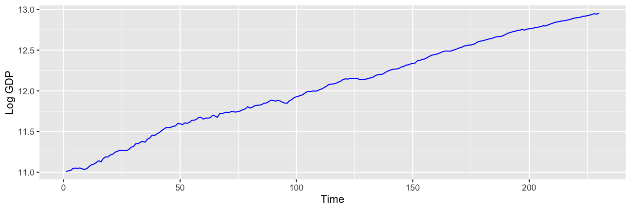Data provided by Tomasz Wozniak in Macroeconometrics ECOM90007

Setting Prior distributions parameters

• Question: "Set the parameters of the natural-conjugate prior distribution and motivate the values that you choose."

• Random Walk with drift process: $logGD{P}_t={\mu }_0+\alpha logGD{P}_{t-1}+u_t$

• $\alpha$=1

• $u_t\sim N(0,{\sigma }^2)$

• $P\left({\sigma }^2\right)\sim I{G}_2(s,\nu )$

• Priors: ${\mu }_0$, $\alpha$, ${\sigma }^2$, s, $\nu$

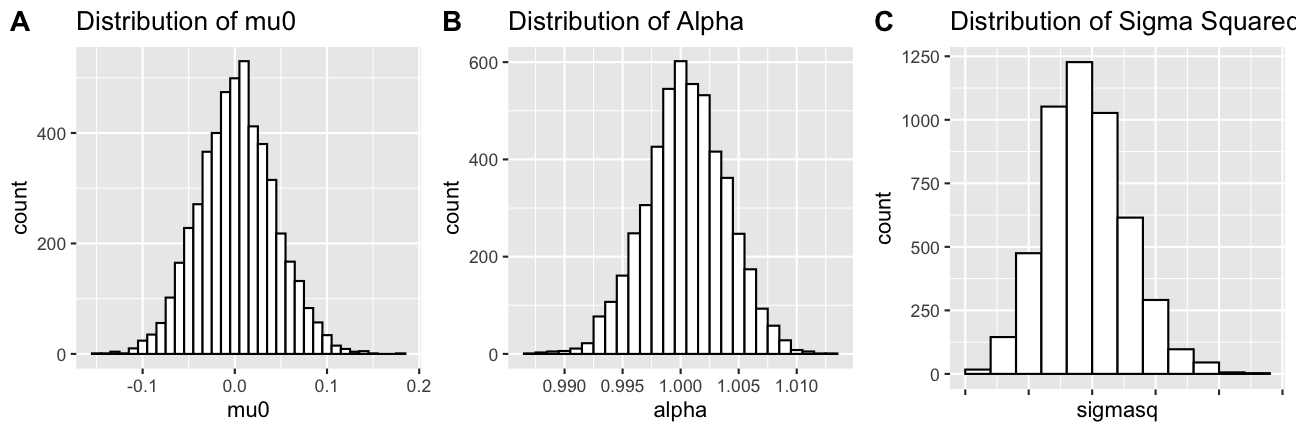
First set of priors testing

• $P(\beta =\left[\begin{array}{c}{\mu }_0\\ \alpha \end{array}\right]|{\sigma }^2)\sim N(\left[\begin{array}{c}0.01\\ 1\end{array}\right],{\sigma }^2\left[\begin{array}{cc}1& 0\\ 0& 10\end{array}\right])$

• The sample mean of ${\mu }_0$ with 5000 draws is 0.0148564 and the variance is 0.011913.

• The sample mean of $\alpha$ with 5000 draws is 0.999454 and the variance is 0.000082.

• The sample mean of ${\sigma }^2$ with 5000 draws is 0.017256 and the variance is 0.0000026.

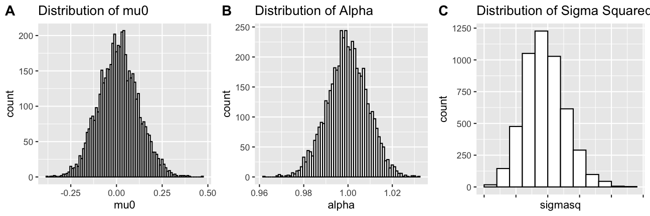
Adjust prior parameters

• $P(\beta =\left[\begin{array}{c}{\mu }_0\\ \alpha \end{array}\right]|{\sigma }^2)\sim N(\left[\begin{array}{c}0.01\\ 1\end{array}\right],{\sigma }^2\left[\begin{array}{cc}0.1& 0\\ 0& 1\end{array}\right])$

• The sample mean of ${\mu }_0$ with 5000 draws is 0.0024582 and the variance is 0.001686.

• The sample mean of $\alpha$ with 5000 draws is 1.00048 and the variance is 0.000012.

• The sample mean of ${\sigma }^2$ with 5000 draws is 0.017258 and the variance is 0.0000026.

Adjust prior parameters

• $P(\beta =\left[\begin{array}{c}{\mu }_0\\ \alpha \end{array}\right]|{\sigma }^2)\sim N(\left[\begin{array}{c}0\\ 1\end{array}\right],{\sigma }^2\left[\begin{array}{cc}1& 0\\ 0& 1\end{array}\right])$

• The sample mean of ${\mu }_0$ with 5000 draws is 0.0114882 and the variance is 0.011913.

• The sample mean of $\alpha$ with 5000 draws is 0.999733 and the variance is 0.000082.

• The sample mean of ${\sigma }^2$ with 5000 draws is 0.017257 and the variance is 0.0000026.

Behind the Scenes

• The sample mean of ${\mu }_0$ with 5000 draws is `r round(mean(blogau$V1),8)` and the variance is `r round(var(blogau$V1),6)` .

• The sample mean of $\alpha$ with 5000 draws is `r round(mean(blogau$V2),6)` and the variance is `r round(var(blogau$V2),8)` .

• The sample mean of ${\sigma }^2$ with 5000 draws is`r round(mean(blogau$sigmasq),6)` and the variance is `r round(var(blogau$sigmasq),8)` .

shh, witchcraft here. Why do I need this chunk to advance to next slide?
@yihui, please send help!

Outputting Plots

R Script

pdf(file="mu0plot.pdf", height=12, width=9)
ggplot(data=blogau, aes(x=V1)) +
    geom_histogram(binwidth=0.01, colour="black", fill="white")+
    ggtitle("Distribution of mu0")+
    xlab("mu0") 
dev.off()

R Markdown

```{r,echo=FALSE,fig.height=12,fig.width=9,dev="pdf"}
ggplot(data=blogau, aes(x=V1)) +
    geom_histogram(binwidth=0.01, colour="black", fill="white")+
    ggtitle("Distribution of mu0")+
    xlab("mu0") 
```

Reference

Alison Hill, June 2019, R-Ladies xaringan theme:  

Professor Chris Skeels, S1 2020,Econometrics ECOM90013, University of Melbourne

Guidotti, E., Ardia, D., (2020), "COVID-19 Data Hub", Journal of Open Source Software 5(51):2376, doi:10.21105/joss.02376.

Tomasz Wozniak, S1 2020, Macroeconometrics ECOM90007, University of Melbourne

Sources

  R Markdown Cheat Sheet

 R Markdown: The Definitive Guide

 Stack Overflow

 RStudio Community

  Workshops: Communicating with Data via R Markdown by Emi Tanaka

Recent Talks about R Markdown on the 2020 RStudio Conference:

 One R Markdown Document, Fourteen Demos by Yihui Xie

 How Rmarkdown changed my life by Professor Rob J Hyndman

  These slides!